Here’s the next part of Nasir’s tutorial on Laplace Transform.
Introduction
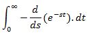
We know that Laplace transformation is a way of transforming integral and differential equations into algebraic equation of s-domain. The expression of Laplace transformation is given as:
In the preceding article we discussed the simulation diagrams. A simulation diagram is basically the pictorial representation of the systems. It shows the functioning of each component and expresses the flow of signals.
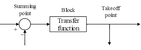
A simple block diagram notation is given as:
For a better understanding of the working of a system we may convert the transform simulation diagrams into flow graphs. A flow graph represents continuous working of a system.
Definition of Flow Graphs
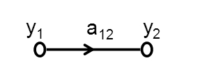
A flow graph is a simpler representation of a block or simulation diagram. It is the graphical embodiment of the association of dependent and independent variables. Below is the example of a simple flow graph:
Elementary Building Blocks of a Flow Graph
Following are the basic elements of a flow graph:
Node:
A node is basically the junction at which the variable is present. It signifies a variable. There are two types of nodes:
- Input Node: a node that has only outgoing branches is called Input node.
- Output Node: a node that has only incoming branches is called an output node.
Path:
The assortment of all the uninterrupted branches, having the same direction is known as a path.
A forwarded Path is a path that initiates from an input node and dismisses at the output node is called a forwarded path. A forwarded path circulates once and only once from each node.
Branch:
The path that joins two nodes is called a branch. A branch mainly consists of a direction and a gain. The Direction shows whether the connection is coming to the node or going out of it.
Loop:
If a path ceases at the node it initiated from, then such a path is called a Loop. Just like a forwarded path a loop doesn’t pass any node more than once.
Loop Gain:
The product of all the branch gains present in a traversing path is called loop gain. To figure loop gain out we use Mason’s gain formula, which states:
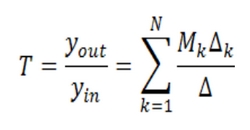
Where,
- N is the total number of forwarded paths between Yin and Yout
- Mk is the gain of the Kth forwarded path
 is the determinant of the graph
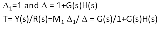
Example 1
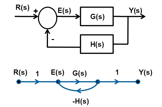
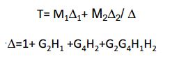
Going from left (R) to the right (Y), we find one forward path M1=G(s).
We are having only one loop which touches the frontward track.
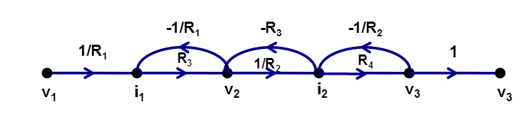
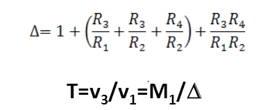
Example 2
Where,
R3R4/R1R2 (two non touching twists along with an increase)
![]() 1=1 (is a forward path touched by each twists)
1=1 (is a forward path touched by each twists)
M1=R3R4/R1R2 (only forward route)
-R3/R1, -R3/R1 and -R4/R2 (three feedback twists having a three increases)
Example 3
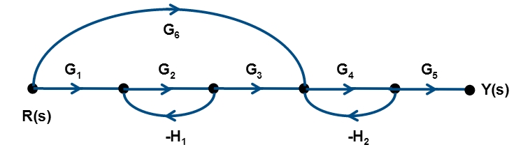
M1= G1G2G3G4G5 and M2= G6G4G5 are forward pathways.
Where,
![]() 1 = 1 (each twist/loop comes in contact with first forward pathway).
1 = 1 (each twist/loop comes in contact with first forward pathway).
![]() 2 = 1+G2H1 (unlike former pathway, first twist doesn’t touch the second pathway).
2 = 1+G2H1 (unlike former pathway, first twist doesn’t touch the second pathway).
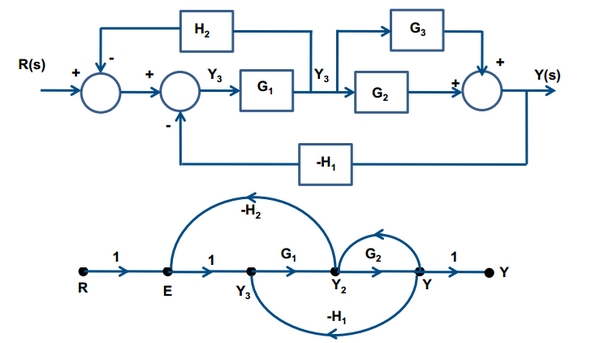
Example 4
To make things more interesting, we are taking a complex example which is not easily solved by clock diagram procedure.
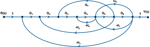
Where,
![]()
are three forward pathways.
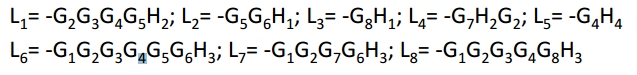
are the increases of feedback twists.
![]()
These are the cofactors involved.
All the twists will touch except for the twists L4 and L7 which will not be touched by L5 and loop L4 which will not be touched by loop L3.
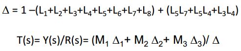
The determinant Δ is given by:
Block Diagram of Signal Flow Graph
By utilizing Mason’s Gain Formula, we will find out the transfer function.
Taking in account the equation written below:
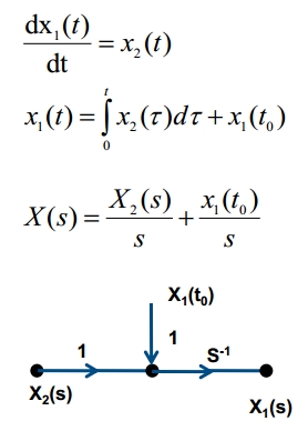
Supposing the initial conditions to be zero, taking the differential equation written below:
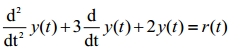
After applying Laplace transform, the result will be:
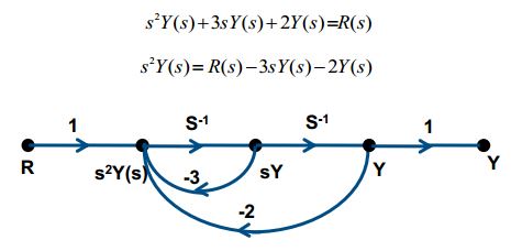
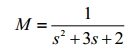
Again we will utilize the Mason’s Gain formula to obtain the transfer function:
Conclusion
So in a nut shell the signal flow graph is a modified form of simulation diagrams. The working of a system can be analyzed with ease if we construct a flow graph with help of the function and simulation diagram.
With flow graphs, the learning part of our Laplace transform comes to an end. We have discussed from the very basics of the Laplace transform and its orientation to its working and simulation diagrams along with the graphs.
It the upcoming at last part of tutorial we will demonstrate maximum number of example we can. This will help us in comprehending the implementation of the Laplace transform. We shall start with some basic functions and then move further to demonstrate the working of each part of this tutorial.
As usual I thank you all for reading my tutorials!
Nasir.