Home › Electrical Engineering Forum › General Discussion › Simulation Diagrams of Laplace Transform
- This topic has 4 replies, 4 voices, and was last updated 9 years, 1 month ago by
 davejo.
-
AuthorPosts
-
2014/08/11 at 10:41 am #11184
 adminKeymaster
Next part of Nasir’s tutorial on laplace transform…
Introduction
Since we have established the fact that we can get the algebraic equations from differential and integral equation by using Laplace transform. To remove the undermined coefficients and variations of parameters, we use helpful Laplace transform and for the matter of fact this is most gainful for the input terms like periodic, pulsive or piecewise.
Having boundary conditions, 0 ≤ t < ∞, we consider a function f (t) and its Laplace integral will be:

Laplace transform has the capability of transforming time domain equations into frequency domain. We can analyze the working of interconnected LTI systems. These analyses are done in s-domain. The analysis can be made easy with the help of simulation diagrams.
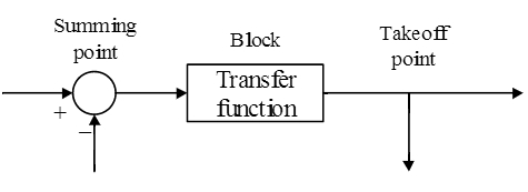
A simulation diagram is basically the pictorial representation of the systems. It shows the functioning of each component and expresses the flow of signals. A simple block diagram notation is given as:

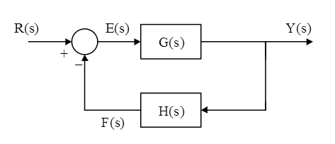
The figure just denotes functioning parts of a sample system. The arrows show the flow signals. The point where all the signals add up, is called summing point and the takeoff works the same ways as in electrical signals. The block contains the transfer function. If we elaborate it a little more, the simulation diagram can be drawn as:

Where,
- U(s) = input (actuating signal)
- R(s) = reference input (command)
- Y(s) = output (controlled variable)
- E(s) = error signal
- F(s) = feedback signal
- G(s) = forward path transfer function
- H(s) = feedback transfer function
Types of stimulation Diagram of Laplace Transform
There are mainly four types of stimulation diagram, which are:
- Single block
- Parallel connection(feed forward)
- Series connection
- Feedback System (closed loop system)
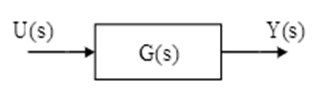
1. Single Block (No Combination):
[caption id="attachment_8245" align="aligncenter" width="334"]
 Y(s) = G(s) U(s)[/caption]
There is just a single block working in the system. In the above system the inputs is represented by U(s), the output is represented by Y(s) and the transfer function of the block by G(s).
2. Parallel Connection (feed forward):
If we connect two systems say, h1(t) and h2(t) in parallel, then its simulation diagram is given as:

The overall impulse response is represented by h (t).

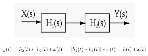
3. Series Connection:
Like parallel combination, consider two systems, h1(t) and h2(t) in series connection, their simulation diagram will be:

The overall impulse response is represented by h (t)

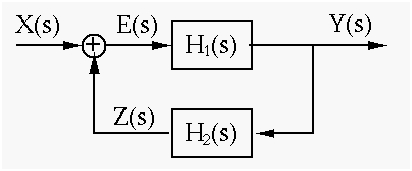
4. Feedback System (closed loop system):

Taking a system constituted of linear time-invariant system. In forward path we have h1(t) and h2(t), another linear time-invariant system in a feedback path. In time domain, we will find the output y (t)

We can write in s-domain

As we know that in time domain it is problematic to solve the equation and finding out the expression for h (t) so that y (t) =h (t)*x (t), also we know that we can solve an algebraic equation painlessly in s-domain to find Y(s).

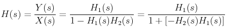
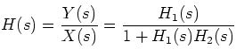
The transfer function can be attained

We ca have either positive or negative feedback. If we have negative feedback then we will have a negative sign in front of h1(t) and H2(t) of the feedback path so that e(t)= x(t) – h2(t) * y(t), also

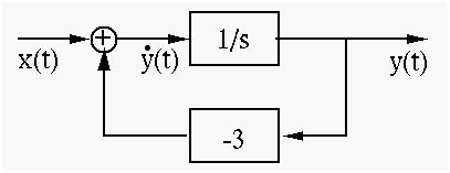
Example 1:
Considering an equation for a system:

We can draw the simulation diagram for the system as below:

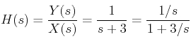
For this system, the equation in s-domain after transformation will be:

with the transfer equation of feedback system, we will compare this equation, we get:
H1(s) = 1/s
and,
H2(s) = 3
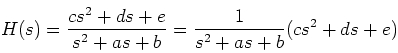
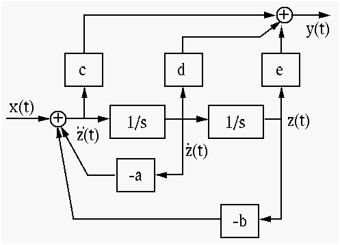
Example 2:
Consider another function whose equation is given by:

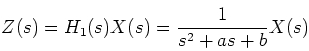
We can represent this as the cascade of two systems:

And
Y(s) = H2(s)A(s) = (cs² + ds + e)Z(s)
The simulation diagram of this system can be demonstrated as:

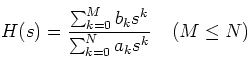
From this diagram, we can generalize the transfer function as:

Conclusion
In this article we dealt with the simulation diagrams and saw how they work for particular systems. When we convert functions from time domain to algebraic equations in s-domain, block or simulation diagrams play a vital role in solving them. It is the pictorial representation of all components of a system and show the flow of signals.
In the upcoming article we will be discussing Flow Graphs of Laplace Transform. That will be the last part of explanations of Laplace transform and then we will move to detailed examples of Laplace transform. So stay stunned for the flow graphs as they are not in any way a least important topic.
Nasir.2014/08/12 at 4:59 pm #13516AnonymousGuestHow the Laplace Transforms and all used in applied engineering???????? Can anyone tell the practical application of LT??
2014/08/23 at 4:22 am #13527mikecollinsParticipantI loved this when undertaking my
Engineering course.2014/08/26 at 11:46 am #13536AnonymousGuestThanks for laying it out so it is so easy to understand, it can be so confusing! I’m trying to study this at the moment. Cheers again
2015/03/03 at 11:39 pm #13654davejoParticipantI was actually trying to simulate a complete block model of Laplace transform on Simulink recently and I faced some issues. Most annoying of which were the variable mismatches but well, that’s Simulink. I actually read both the examples and the transform of a second order equation is now a bit more easy for me to understand.
-
AuthorPosts
 Y(s) = G(s) U(s)[/caption]
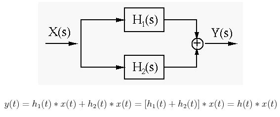

- You must be logged in to reply to this topic.