Hi everybody, it’s Mile, your fellow electrical engineer from Macedonia. I’m glad to discuss about efficient transformer design with you all today and I hope you’ll like my essay.
Energy efficiency is closely connected to the living environment and is one of the most important questions today. According the laws and regulations, it is important to use energy efficient equipment in the power systems, because of the benefits like energy saving.
Distributive transformers are one of the elements in the power system that generate the power losses, so decreasing those losses will result with higher economic and ecological gain. Decreasing the losses is a complex question and the only solution is careful planning and optimal design of the transformer.
In this article, a modern and practical optimization solution is presented to decrease power losses. The test transformer is with the following parameters: S=50 kVA, Un=20/0,4 kV, and connection type Yzn5.
Mathematical model of the xformer
In general, the losses in the transformer are divided in two components: Losses in copper and non-load losses. Non load losses arise from the energy of the magnetic field which is needed to maintain the magnetic flux in the transformer core.
These losses are constant and are not connected to the load increase. Copper losses are proportional to the square of the load current. Optimal design is based on minimizing the total losses and is adapted through mathematical model of the transformer. There are actually 9 variables for the mathematical model starting from x1-x9, which represent the geometrical dimensions of the transformer and some electric or magnetic values.
The total losses are actually mathematical function of those values. The mathematical expression is:
Z = Total losses = f [x1 x2 x3 x4 x5 x6 x7 х8 x9] Т
x1=Bm (1,65 – 1,75) – induction (T)
x2=λ (2,2 – 2,5) – height and diameter ratio (/)
x3=q1 (2870000 – 3500000) – current density in HV winding (A/m2)
x4=q2 (3340000 – 3500000) – current density in LV winding (A/m2)
x5=γ (0,14 – 0,2) – ratio of non load and short circuit losses (/)
x6=υ2 (0,01 – 0,02) –distance between LV winding and the yoke (m)
x7=k (0,004 – 0,006) – distance between pillar and LV winding (m)
x8=υ1 (0,02 – 0,03) – distance between HV winding and the yoke (m)
x9=ξ (0,007 – 0,015) – distance between LV and HV winding (m)
We are going to use the Pattern Search technique for our purposes. Minimizing the losses in the transformer, will result in achieving greater energy efficiency.
According the expression for the total losses we are going to enter the following values for our test case.
x0=[1,675 2,393 2870000 3420000 0,181 0,01 0,006 0,025 0,014]
Additional nonlinear limitations that we must take into consideration are:
120≤mfe[x]≤140,7 , mfe – weight of transformer core (kg)
40≤mCu[x]≤50,04 , mCu – weight of the coils (kg)
900≤Pcu[x]≤1187 , Pcu – nominal losses in copper (W)
190≤Pfe[x]≤240 , Pfe– nominal losses in steel (W)
3.6≤uk[x]≤4.4 , uk– short circuit voltage (%)
In the optimization process there is a request regarding the weight of the active parts of the transformer. That weight should not be greater than the weight of the active parts of the original transformer. Also, there is a limitation regarding the short circuit voltage. It should not be greater than 10% of those maximal 4%, according the IEC 60067 standard.
Transformer design optimisation results
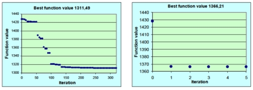
As we can see on picture 1, when there are no non-linear limitations, we receive lower values for the function that is minimizing.
Picture 1. Convergence optimization process
Based on the gathered results, we started building the new transformer in several stages, as you can see on picture 2.
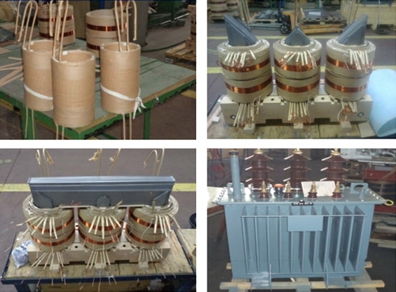
Picture 2. Transformer building stages
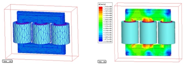
Picture 3. ANSOFT MAXWELL analysis
For the purpose of analysis we made an computer simulation for the prototype transformer, which is presented on picture 3. Comparison between the original and the prototype transformer is presented in table 1.
|
|
mFe (kg) | mCu (kg) | PFe (W) | Pcu75˚ (W) | Pγ (W) | h (/) | uk (%) |
| Original | 140,7 | 50,4 | 240 | 1187 |
1428 |
97,223 | 3,94 |
| Prototype | 135,9 | 46,29 | 228 | 1138 | 1366 | 97,341 | 3,66 |
| Deviation | -3,41 | -7,49 | -5 | -4,13 | -4,34 | +0,121 | -7,1 |
Table 1. Comparison of results
Conclusion
From the previously stated, we can conclude that the mathematical model and the optimization technique gave good results, which we can see from the results in table 1. The losses in copper and steel, and the total losses in the xformer are lowered, and thus the energy efficiency of the xformer is increased.
Also, a significant achievement has been made regarding the weight of the active parts of the xformer, which is important from economical aspect, because we are drastically lowering the price of the xformer.
Thank you everybody for your attention,
Mile.
If you have something to ask or a remark, do not hesitate to post a comment below!